Z-projections: finding the best focused plane
In the previous tutorial, we learned the basics of projections in the Z-plane. We highlighted the importance of finding the central, focused slice to select a projection range that falls within the focal plane of our sample. Doing this manually can be tedious, but what if I told you we can automate that step? Let’s learn how to set up a script to automatically detect the best-focused slice.
Import packages and image
For this tutorial we will need the following packages:
from skimage import data
import numpy as np
import matplotlib.pyplot as plt
import cv2
And then we import also the image of the nucleis that we have used before.
image = data.cells3d()
image_nuclei = image [:,1,:,:] # to get the nuclear channel
How do we find the best focused slice?
To automatically detect the best-focused plane, we rely on the mathematical parameters of our image. There are several strategies that we can use, let’s test some of them.
Using pixels standard deviation
For fluorescent images, the standard deviation (SD) of pixel intensities is a reliable indicator. SD measures how spread out the values are in a dataset—in this case, the pixel intensities. In a perfectly focused image, the boundaries of structures are sharp, resulting in a significant difference in intensity between pixels in the background and those within the cell, which leads to a higher SD for the entire image. Conversely, if the image contains blur, pixels near the edges of structures will have more averaged intensities, resulting in a lower SD for the image.
Let’s code!
We’re going to calculate the standard deviation (SD) for each slice and compare the results. To do this, we’ll need to split the stack into individual 2D slice images. Remember for loops? We’ll use one to go through each slice in the stack and calculate its SD.
z_values = [] # Empty lists to store results
sd_values = []

for z in range (image_nuclei.shape[0]):
    slice_2D = image_nuclei[z,:,:] # Extract the 2D image
    sd = slice_2D.std()  # Calculate the standard deviation of the 2D slice

    # Store the results
    z_values.append(z)
    sd_values.append(sd)
Great! Let’s create a graph to see how the standard deviation values vary across the Z-planes. This will help us visually identify the slices with the highest focus by observing the SD trends along the Z-axis.
# Plot the SD values across Z
plt.plot(z_values, sd_values, marker='8', linestyle='-', color='darkorchid')
plt.xlabel("Z-axis (Slice Index)")
plt.ylabel("Standard Deviation (SD)")
plt.title("Standard Deviation Across Z-axis Slices")
plt.show()
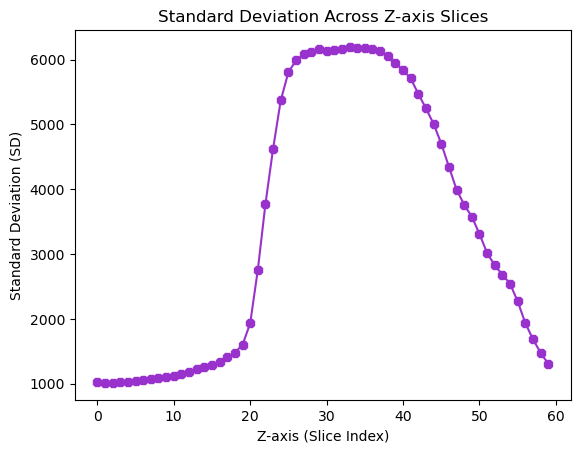
Looking at the graph, we can see that the slices with the highest values are approximately between 27 and 38. We will consider the best focused slice as the one with the highest SD value.
sd_values_array = np.array(sd_values) # to look for the highest value we need to convert the list into an array
maxsd_index = sd_values_array.argmax() # to look for the index position with the highest sd value
print(maxsd_index)
33
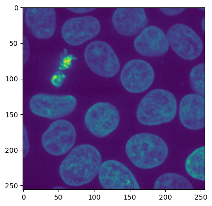
It appears that slice 33 is the one with the best focus! Let’s take a look 👀
# Visualize the image
fig, ax = plt.subplots(1, 1, figsize=(15, 5))
ax.axis('off') # remove the axis of the figure
plt.imshow(image_nuclei[33,:,:])
<matplotlib.image.AxesImage at 0x13b4dfeb0>
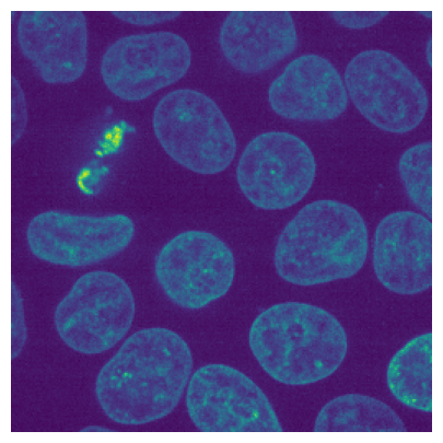
It seems pretty decent!
This method works well for fluorescent images, but it’s not suitable for brightfield images because the pixel intensities in brightfield microscopy primarily vary at the edges of structures rather than throughout the entire slice. Let’s look for a universal method.
Using advanced mathematical operators: variance of Laplace
We will explore the application of the variance of the Laplace operator, a powerful mathematical tool often used in image processing. The Laplace operator enhances features in an image by emphasizing edges. The better focused the image is, the more clearly the edges will be defined, resulting in higher Laplacian variance.
lp_values = [] # Empty lists to store results

for z in range (image_nuclei.shape[0]):
    slice_2D = image_nuclei [z,:,:] # Extract the 2D image
    laplacian = cv2.Laplacian(slice_2D, cv2.CV_64F, ksize=9) #max kernel size of 31
    # Calculate the variance of the Laplacian
    variance = laplacian.var()

    # Store the results
    lp_values.append(variance)
Let’s visualize a frame that we know is unfocused along with a focused one before after the Laplacian transformation.
# Visualize the raw and Laplacian images for z=19 and z=34
fig, axes = plt.subplots(1, 4, figsize=(15, 5))

# Display the raw and Laplacian of the image at z=19
axes[0].imshow(image_nuclei[19, :, :])
axes[0].axis('off')  # Remove axis
axes[0].set_title("Raw image for z=19")

axes[1].imshow(cv2.Laplacian(image_nuclei[19, :, :], cv2.CV_64F, ksize=9), cmap='gray')
axes[1].axis('off')  # Remove axis
axes[1].set_title("Laplacian for z=19")

# Display the raw and Laplacian of the image at z=34
axes[2].imshow(image_nuclei[34, :, :])
axes[2].axis('off')  # Remove axis
axes[2].set_title("Raw image for z=34")

axes[3].imshow(cv2.Laplacian(image_nuclei[34, :, :], cv2.CV_64F, ksize=9), cmap='gray')
axes[3].axis('off')  # Remove axis
axes[3].set_title("Laplacian for z=34")

plt.show()
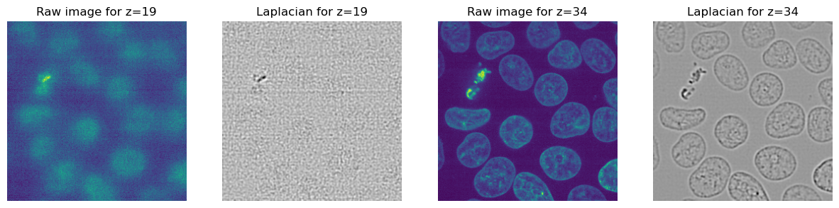
The differences are clear: the transformation effectively detects borders when the image is well-focused, resulting in a higher pixel variance.
Let’s look now for the best focused slice:
lp_values_array = np.array(lp_values) # to look for the highest value we need to convert the list into an array
maxsd_index = lp_values_array.argmax() # to look for the index poition with the highest sd value
print(maxsd_index)
34
34! Looks like there’s not much difference between using the Laplacian transformation and the standard deviation method to check focus—they’re pretty close!
Let’s compare the values of both methods across the Z.
# Plot the Laplacian variance values and SD across Z
fig, ax1 = plt.subplots()

color = 'darkorchid'
ax1.set_xlabel('Z-axis (Slice Index)')
ax1.set_ylabel("Standard Deviation (SD)", color=color)
ax1.plot (z_values, sd_values, marker=".", color=color)

ax2= ax1.twinx() # copy the ax1

color = 'forestgreen'
ax2.set_xlabel('Z-axis (Slice Index')
ax2.set_ylabel("Variance of Laplace", color=color)
ax2.plot (z_values, lp_values, marker="x", color=color)


#plt.plot(z_values, sd_values, marker='8', linestyle='-')
#plt.plot (z_values, lp_values, marker= 'x', linestyle='dotted')
#plt.xlabel("Z-axis (Slice Index)")
#plt.ylabel("Laplacian Variance (SD)")
#plt.title("Standard Deviation Across Z-axis Slices")
plt.show()
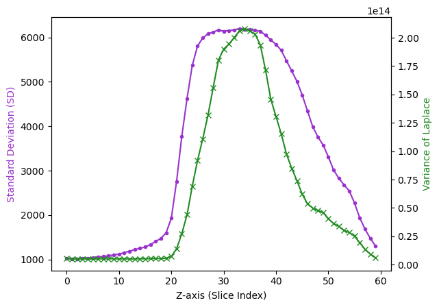
As you can see, Laplacian variance is a more sensitive method for detecting focus.
Let’s wrap up!
Now we can update the function created in the previous section so it also automatically detects the best focused plane and creates the desired projection.
def focus_detection_projection(image, stack_width, projection_type='max', axis = 0):
    """
    Detects the best focused slice of a z-stack and computes the specified projection (max, min, or average) of a 3D image stack.

    Parameters:
    -----------
    image_3d : numpy.ndarray
        A 3D array representing the image stack (z, x, y).

    stack_width : Determine how many slices would be included in the projection. e.g. if the parameter is set to 3 it will take best focused
    slice, 3 above and 3 below. total of 7.


    projection_type : str, optional, default='max'
        The type of projection to compute. Options are:
        - 'max' for Maximum Intensity Projection
        - 'min' for Minimum Intensity Projection
        - 'avg' for Average Intensity Projection
        - 'none' for returning the best focused slice.

    axis : int, optional, default=0
        The axis along which to compute the projection (0 = , 1 = , 2 = ).

    Returns:
    --------
    projection : numpy.ndarray
        The 2D projection image.
    """
    lp_values = [] # Empty lists to store results
    z_values = []

    for z in range (image.shape[axis]):
        slice_2D = np.take(image, indices=z, axis=axis) # Extract the 2D image
        laplacian = cv2.Laplacian(slice_2D, cv2.CV_64F, ksize=9) #max kernel size of 31
        # Calculate the variance of the Laplacian
        variance = laplacian.var()

        # Store the results
        lp_values.append(variance)
        z_values.append(z)

    lp_values_array = np.array(lp_values) # to look for the highest value we need to convert the list into an array
    best_focused_index = lp_values_array.argmax() # to look for the index position with the highest sd value

    # Select the range of slices around the best-focused index
    start_index = max(0, best_focused_index - stack_width)
    end_index = min(image.shape[axis], best_focused_index + stack_width + 1)

    # Use np.take to extract the slices along the specified axis
    indices = list(range(start_index, end_index))
    image_2project = np.take(image, indices=indices, axis=axis)

    # Choose the projection type
    if projection_type == 'max':
        projection = np.max(image_2project, axis=0)
    elif projection_type == 'min':
        projection = np.min(image_2project, axis=0)
    elif projection_type == 'avg':
        projection = np.mean(image_2project, axis=0)
    elif projection_type == 'none':
        projection = image[best_focused_index, :, :]
    else:
        raise ValueError("Invalid projection type. Choose from 'max', 'min', 'avg', or 'none'.")

    return projection
Let’s try it!
projection = focus_detection_projection(image_nuclei, 5, projection_type='avg', axis=0)

plt.imshow(projection)
<matplotlib.image.AxesImage at 0x13b8d22c0>
If you’ve made it this far, leave a reaction! 🎉